속도 프로파일과 탄성파 트레이스 추출하여 그리기
속도모델에서 프로파일을 추출하여 깊이에 따라 속도 그림을 그려보겠습니다. 이진 형식의 속도파일에서 텍스트 파일로 프로파일을 추출한 후 그리는 방법과 이진 속도파일을 직접 읽어서 그리는 방법을 살펴보겠습니다. 참고로, 탄성파 공통송신원모음 등에서 트레이스를 추출하여 그리는 과정 또한 동일합니다.
텍스트 파일로 추출하여 그리기
바이너리 파일에서 프로파일 또는 트레이스를 추출하기 위해
gpl 라이브러리의
gplTracePick 프로그램을 사용하겠습니다. 이차원 단면(속도모델, 공통송신원모음 등)에서 세로 방향 트레이스를 추출할 때 사용하는
프로그램입니다. (가로방향 트레이스는 gplHTracePick 프로그램을 이용하면 됩니다.) 이 프로그램을 그냥 실행하면 아래와 같은
도움말이 나옵니다.
1
2
%%sh # 이 글을 쓰고 있는 jupyter notebook에서 shell 명령을 실행하기 위한 magic command입니다.
gplTracePick # 실제 터미널상에서 실행하는 명령어
 Gpl trace picker
 Required parameters:
     [i] n1=            : # of grids in fast dimension
     [s] fin=           : input binary file
     [s] fout=          : output binary file
     [i] pick=          : (=first), first pick (1~n2)
 Optional parameters:
     [i] last=first     : last pick (pick~n2)
     [i] step=1         : pick step
     [f] d1=1.0         : grid size
     [i] n2=calc        : # of grids in slow dimension
     [s] type=f         : data type [ifdcz]
     [s] otype=a        : output type [ab] (ascii/binary)
위에서 n1, fin, fout, pick은 프로그램 실행시 필수적으로 넣어줘야 하는 값입니다.
n1은 세로 방향(fast dimension) 격자수fin은 입력 파일 이름fout은 출력 파일 이름pick은 추출하고자하는 가로 방향(slow dimension) 격자 번호입니다. 격자 번호는 1번부터 시작합니다.
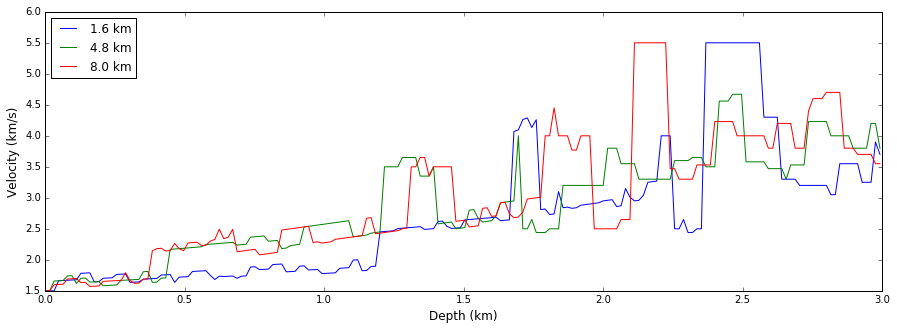
Marmousi 속도모델(nx=576, ny=188, h=0.016 km)에 대해 1.6 km 지점(격자번호 101)에서 시작하여 3.2 km 간격(200개 격자 간격)으로 3개의 속도 프로파일을 추출한다면 아래와 같이 실행할 수 있습니다.
1
2
%%sh
gplTracePick n1=188 d1=0.016 fin=marm16km.bin fout=vel_profile.txt pick=101 step=200 last=501
 n2=         576


     n1=188
     d1=0.016
     fin=marm16km.bin
     fout=vel_profile.txt
     pick=101
     step=200
     last=501
그 때 결과물은 아래와 같습니다. 첫 번째 열은 깊이 정보, 두 번째부터 네 번째 열까지는 추출한 속도 프로파일 정보입니다(1.6 km, 4.8 km, 8.0 km).
1
2
%%sh
head vel_profile.txt
   0.00000000       1.50000012       1.50000012       1.50000012
   1.60000008E-02   1.50000012       1.50000012       1.50000012
   3.20000015E-02   1.50000012       1.65800011       1.59800005
   4.80000004E-02   1.66200006       1.66200006       1.60200012
   6.40000030E-02   1.66600013       1.66600013       1.60600019
   8.00000057E-02   1.67000008       1.73999715       1.69000006
   9.60000008E-02   1.67400002       1.74399781       1.69400012
  0.112000003       1.67800009       1.61800003       1.69800007
  0.128000006       1.78200006       1.70200002       1.63200009
  0.144000009       1.78600013       1.70600009       1.63600004
텍스트 파일로 추출한 결과는 gnuplot과 같은 프로그램을 이용해 빠르게 확인해볼 수 있습니다. 여기서는 파이썬의 Matplotlib을 이용하여 위의 속도 프로파일을 그려보겠습니다.
1
2
3
%matplotlib inline
import matplotlib.pyplot as plt
import numpy as np
1
2
trc=np.loadtxt("vel_profile.txt")
trc.shape
(188, 4)
1
2
3
4
5
6
7
8
9
10
h=0.016
fs='large'

plt.figure(figsize=[15,5])
for i,ix in enumerate([100,300,500]):
    plt.plot(trc[:,0],trc[:,i+1],label="{0} km".format(ix*h))

plt.legend(loc="upper left",fontsize=fs)
plt.xlabel("Depth (km)",fontsize=fs)
plt.ylabel("Velocity (km/s)",fontsize=fs)
<matplotlib.text.Text at 0x10cc66c88>
이진 파일을 직접 읽어서 그리기
이번에는 파이썬에서 이진 형식의 속도모델 파일을 직접 읽어서 그려보겠습니다.
1
2
3
4
nx=576
ny=188
vel=np.fromfile("marm16km.bin",dtype=np.float32)
vel.shape=(nx,ny)
1
2
3
4
5
6
7
8
9
10
11
h=0.016
fs='large'
depth=np.arange(ny)*h

plt.figure(figsize=[15,5])
for ix in [100,300,500]:
    plt.plot(depth,vel[ix,:],label="{0} km".format(ix*h))

plt.legend(loc="upper left",fontsize=fs)
plt.xlabel("Depth (km)",fontsize=fs)
plt.ylabel("Velocity (km/s)",fontsize=fs)
<matplotlib.text.Text at 0x10d13dd30>

참고로, 파이썬은 배열 인덱스가 0번부터 시작하기 때문에 가로방향 100, 300, 500번 속도 프로파일을 가져다가
그렸습니다(gplTracePick을 이용하는 앞의 예제에서는 101, 301, 501번 격자 위치에서 추출했죠).
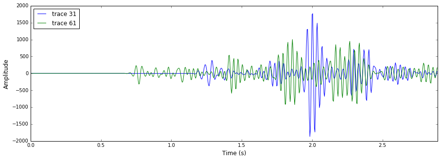
탄성파 트레이스 그리기
공통송신원모음에서 탄성파 트레이스를 추출하여 그리는 과정은 속도모델에서 프로파일을 추출하여 그리는 경우와 동일합니다. 아래는 샘플 개수가 723개, 샘플링 간격 4 ms, 트레이스가 96개인 공통송신원모음 파일(marm3000.bin)에서 31번째와 61번째 트레이스를 그리는 예제입니다.
1
2
3
4
5
ntr=96
ns=723
dt=0.004
trc=np.fromfile("marm3000.bin",dtype=np.float32)
trc.shape=(ntr,ns)
1
2
3
4
5
6
7
8
9
10
fs='large'
time=np.arange(ns)*dt

plt.figure(figsize=[15,5])
for itr in [30,60]:
    plt.plot(time,trc[itr,:],label="trace {0}".format(itr+1))
plt.legend(loc="upper left",fontsize=fs)
plt.xlabel("Time (s)",fontsize=fs)
plt.ylabel("Amplitude",fontsize=fs)
plt.xlim([0,ns*dt])
(0, 2.892)